Extracting Trees from Baltimore LiDAR — 2008 and 2014

The Data

Both tiles come from NOAA's Coastal LiDAR program, distributed as Cloud-Optimized Point Cloud (COPC) LAZ files. The tile index was browsed in QGIS to select an overlapping area of downtown Baltimore across both survey years.

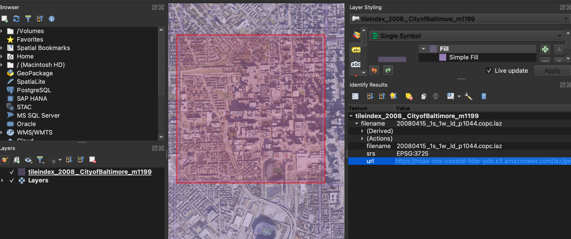
Both tiles cover roughly 1.5–1.6 km² in UTM zone 18N, with vertical datum NAVD88. The CRS differs between years: the 2008 survey uses NAD83(NSRS2007) (EPSG:3725) while 2014 uses the updated NAD83(2011) realization (EPSG:6347).

Inspecting the files with laspy revealed that neither dataset uses standard vegetation classification codes (3 = low, 4 = medium, 5 = high vegetation). Tree extraction had to be derived entirely from geometry.

Architecture Overview

The stack runs entirely on a single home server — a CPU-only Intel i3 machine with 3.7GB of RAM running Debian 13. There is no GPU and no cloud dependency. Both datasets run through the same pipeline into separate PostGIS tables.

Ingestion: LAZ → PostGIS

Each dataset has its own pair of PostGIS tables — points / points_2014 and trees / trees_2014 — with geometry columns typed to the correct EPSG for each year. points stores every point as a PointZ geometry alongside intensity, classification, return metadata, and a hag column populated in the next step.

CREATE TABLE points (
    id              SERIAL PRIMARY KEY,
    geom            GEOMETRY(PointZ, 3725),  -- 6347 for 2014
    intensity       INTEGER,
    classification  SMALLINT,
    return_number   SMALLINT,
    num_returns     SMALLINT,
    gps_time        DOUBLE PRECISION,
    hag             DOUBLE PRECISION
);

Bulk insertion used psycopg2's execute_values in batches of 50,000 rows. One early issue: psycopg2 cannot adapt numpy.int64 directly — all numpy scalars must be cast to Python native types. With that fix: 3.5M points in 145 seconds for 2008, 13.2M points in 603 seconds for 2014.

Height Above Ground

Raw LiDAR Z values are absolute elevation (NAVD88 metres). Each point needs its elevation relative to the local ground surface — Height Above Ground (HAG) — to make vegetation height meaningful independent of terrain.

The approach: rasterize the class 2 ground points onto a 1-metre grid using scipy.stats.binned_statistic_2d, fill empty cells with nearest-neighbour interpolation via scipy.ndimage.distance_transform_edt, then evaluate the resulting RegularGridInterpolator at every point's XY position.

stat, _, _, _ = binned_statistic_2d(
    gx, gy, gz, statistic='mean', bins=[x_bins, y_bins]
)
mask = np.isnan(stat)
indices = distance_transform_edt(mask, return_distances=False, return_indices=True)
stat = stat[tuple(indices)]

interp = RegularGridInterpolator(
    (x_centers, y_centers), stat,
    method='linear', bounds_error=False, fill_value=None
)
hag = z - interp(np.column_stack([x, y]))

The 2008 DEM used 1.14M ground points on a 1644×1644 grid; HAG ranged −84 to +111m. The 2014 DEM used 2.0M ground points on a 1500×1501 grid; HAG ranged −90 to +75m. Negative values in both are noise or underwater returns and are filtered downstream.

Tree Segmentation

Without pre-classified vegetation, trees were identified by two geometric filters applied to the full point cloud:

• HAG > 2m — eliminates ground-level returns
• num_returns > 1 — multi-return pulses indicate the laser penetrated a canopy. Buildings and pavement return a single pulse from a hard surface.

The 2014 pipeline additionally excludes class 17 (bridge deck) and class 18 (high noise), which together account for nearly 60% of that dataset and would contaminate the vegetation candidates if left in.

mask = (hag > 2.0) & (num_returns > 1) & (cls != 2) & (cls != 7)
# 2014 also excludes: & (cls != 17) & (cls != 18)

labels = DBSCAN(
    eps=3.0, min_samples=10,
    algorithm='ball_tree', n_jobs=-1
).fit_predict(np.column_stack([cx, cy]))

Clusters with fewer than 20 points or HAG max above 40m are discarded as noise or building remnants. Each surviving cluster becomes a tree record: centroid, convex hull crown polygon, point count, and height statistics.

2008 Results

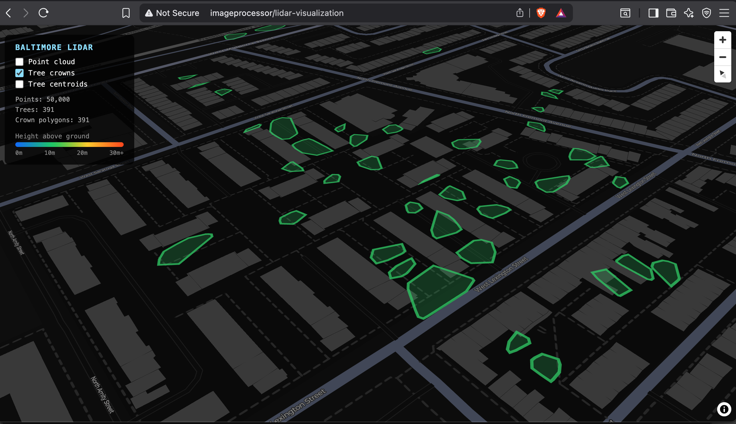
Tree crowns cluster along what appear to be park strips, street medians, and open lots. The coverage is sparse but spatially coherent — trees are not randomly distributed across the tile. The April survey date means deciduous trees were still largely bare, which likely suppressed multi-return counts and reduced the number of trees detected.

2014 Results

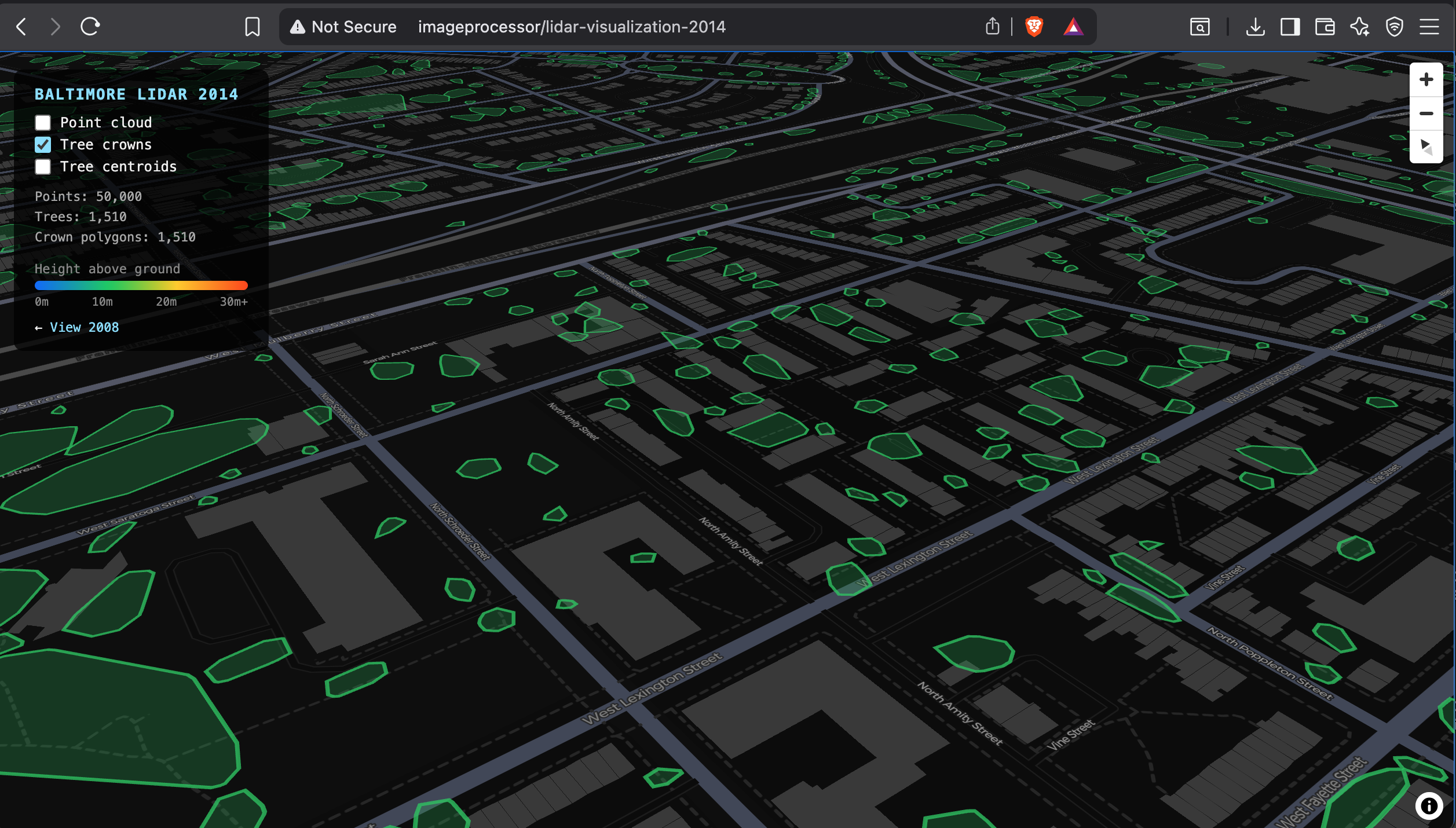
The 2014 tile shows substantially more tree coverage — 1,510 crowns vs 391 in 2008, nearly 4×. The higher point density (13.2M vs 3.5M points) means more canopy returns per tree, making individual trees easier to resolve as distinct clusters. The December survey date, however, means leaf-off conditions again, which would have suppressed some multi-return signal in deciduous trees.

Class 17 "Bridge deck" accounts for 40.5% of the 2014 cloud, likely reflecting harbor infrastructure captured in this tile that was absent or classified differently in 2008. Class 18 "High noise" at 18.4% — 2.4 million points — is consistent with water surface returns from the inner harbor: LiDAR reflects poorly off water and produces scattered, high-elevation spurious returns.

Web Visualization

Each dataset has its own deck.gl viewer, linked to each other, served by a single FastAPI app behind nginx. Both viewers use the same three-layer structure: a sampled point cloud colored by HAG, convex hull crown polygons, and clickable tree centroids.

• http://imageprocessor/lidar-visualization — 2008 survey
• http://imageprocessor/lidar-visualization-2014 — 2014 survey

The FastAPI backend reprojects coordinates from each year's native CRS to WGS84 on the fly using pyproj. The /api/points endpoint uses ORDER BY random() LIMIT n for sampling directly in PostGIS, keeping the API stateless and the payload to a fixed size regardless of dataset scale.

transformer_2008 = Transformer.from_crs("EPSG:3725", "EPSG:4326", always_xy=True)
transformer_2014 = Transformer.from_crs("EPSG:6347", "EPSG:4326", always_xy=True)

@app.get("/api/points")
def get_points(n: int = 50000):
    return fetch_points("points", transformer_2008, n)

@app.get("/api/2014/points")
def get_points_2014(n: int = 50000):
    return fetch_points("points_2014", transformer_2014, n)

Infrastructure

The machine (imageprocessor.lan) is a repurposed desktop running Debian 13 Trixie on an Intel i3-6100T with 3.7GB RAM. It is CPU-only — no GPU — and connected to the network over WiFi (Intel 8260, −40 dBm signal). PostGIS runs in a Docker container with its data volume on the host filesystem.

• Python 3.13.5, virtualenv at ~/lidar/venv
• PostgreSQL 17 + PostGIS 3.5 — postgis/postgis:17-3.5 Docker image
• nginx 1.26 reverse proxy, uvicorn on port 8000
• SSH key auth, ian user with NOPASSWD sudo

One setup complication: the machine had its system clock set to September 2025, causing apt to reject the Debian 13 repository with a "not live until" error. Correcting the clock with timedatectl set-ntp true resolved it immediately.

What This Stack Demonstrates

• End-to-end LiDAR processing pipeline from raw LAZ to browser visualization
• PostGIS as a spatial store for 3D point cloud data and derived geometries
• Ground DEM construction via raster binning and nearest-neighbour fill
• Multi-return filtering as a low-cost vegetation indicator without ML
• DBSCAN for individual tree crown segmentation on XY projections
• Running the same pipeline on two survey years to produce a consistent comparison
• FastAPI + deck.gl for serving spatial data with on-the-fly CRS reprojection
• systemd + nginx for reliable local network service hosting
• CPU-only geospatial processing at 13M+ point scale without a GPU